Determining Polar Axis Alignment Accuracy
by Frank Barrett
2nd Edition 9/21/2016
Abstract: In order to photograph dim celestial objects, long exposures on the order of minutes or hours are required. To perform this process successfully the mount needs to rotate to compensate for the earth’s rotation. To achieve this, the mount’s rotational axis must be critically aligned parallel to the earth’s rotational axis. This process is known as polar axis alignment. Two primary questions are answered in this article relative to polar axis alignment. First, “How can I determine the magnitude of my polar alignment error?”, and second, “What is the required tolerance for alignment error for a given imaging session?”
Drift Alignment Overview
Before we examine the details of polar axis alignment it is beneficial to review the drift alignment method. Drift alignment is a very popular method for polar alignment of equatorial mounts particularly when very high accuracy is needed. The method requires that the scope point at a carefully selected reference star. If the star drifts in declination it indicates misalignment in the mount’s rotational axis.
Here is how the procedure works. To measure and adjust the azimuth axis, monitor a star near the intersection of the celestial equator and the meridian. If the star drifts north the mount is pointing too far west. A southern drift indicates the mount is pointing too far east. Likewise, to measure and adjust the altitude axis, monitor a star in the east near the celestial equator. If the star drifts north the mount is pointing too high. A southern drift indicates the mount is pointing too low. In each case the rate of drift is indicative of the magnitude of the error and the adjustment required for correction. Note that the drift direction should be reversed in the southern hemisphere or if an altitude reference star is selected in the west. The procedure is repeated on each axis until no discernable drift is observed or, as this article will show, until the remaining alignment error is within the tolerance required for the imaging session. [1]
Hook’s Equations
The undesirable consequence of a poor alignment is that a guided image may show field rotation centered on the guide star. It is this field rotation that we seek to eliminate by carefully aligning the polar axis of our mount. In an article in the February 1989 issue of the Journal of the British Astronomical Association, Richard Hook derived a number of equations which showed how far a star would drift on an unguided mount and the alignment tolerance required to hold field rotation to within a given limit. We will use Hook’s equations to answer our primary questions and then take a closer look into these equations to understand how various factors of the imaging process affect the field rotation. [2]
Question 1: What is the magnitude of my polar alignment error?
With the drift method we have a means of detecting declination drift for each polar alignment axis. The question here is: “Can I determine the polar axis misalignment given an accurate measure of the declination drift?” The answer is: Yes! Hook showed that the declination drift was related to the angle of alignment error as follows:
![]()
Where:
![]() is the declination
drift in degrees
is the declination
drift in degrees
![]() is the time of
drift in minutes
is the time of
drift in minutes
![]() is the
declination of the drift star used
is the
declination of the drift star used
![]() is the alignment
error in radians
is the alignment
error in radians
Since the drift error is typically very small it is more convenient to express the drift in arc seconds:
![]()
Solving for ![]() gives:
gives:
![]()
We generally like to express alignment errors in arc minutes, so to convert radians to arc minutes we arrive at:
![]()
So:
![]() (1)
(1)
Where:
![]() is the
alignment error in arc minutes
is the
alignment error in arc minutes
![]() is the declination
drift in arc seconds
is the declination
drift in arc seconds
![]() is the time of
drift in minutes
is the time of
drift in minutes
![]() is the
declination of the drift star used
is the
declination of the drift star used
For example, given: ![]() = 20.5”,
= 20.5”, ![]() = 10 minutes, and
= 10 minutes, and ![]() = 35 degrees:
= 35 degrees:
![]()
Measuring the declination drift
The declination drift can be estimated visually using a well-calibrated reticule eyepiece. More accurate measurements can be achieved with camera assisted methods. For example, autoguiding software works by taking images of a reference star and measuring the distance of that star from a reference pixel in the image. Corrections are sent to the mount to reposition the star at the reference point and the process is repeated throughout the duration of the exposure. Most autoguiding software can operate in a mode where the star offset is reported without any correction made. This is perfect for our purposes since the offset in the declination axis over time is the measurement in which we are interested. The image exposure time should be long enough to average out atmospheric seeing effects or a reasonable estimate can be obtained by averaging the last few measurements. Also note that a requirement of Equation (1) is that the drift needs to be expressed in arc seconds. If the autoguiding software reports the error in pixels the needed conversion is as follows:
![]() (2)
(2)
Where:
![]() is the calculated
drift in arc seconds
is the calculated
drift in arc seconds
![]() is the measured
drift in pixels
is the measured
drift in pixels
![]() is the pixel
size in microns
is the pixel
size in microns
![]() is the focal
length in mm
is the focal
length in mm
A more thorough treatment of declination drift measurement techniques is given in [4].
Question 2:
How do I know when my alignment is “Good Enough”?
By means of Equation (1) we know the alignment error based on the declination drift. So how good is good enough? Hook also answered that question by showing that the maximum tolerable error is related to the declination of the target, the elapsed time of the exposure, the effective focal length of the instrument, and the angle between the guide star used and the opposite edge of the field as follows:
![]()
Where:
![]() is the maximum
permitted alignment error in degrees
is the maximum
permitted alignment error in degrees
![]() is the declination
of the target in degrees
is the declination
of the target in degrees
![]() is the time of
exposure in minutes
is the time of
exposure in minutes
![]() is the focal
length in millimeters
is the focal
length in millimeters
![]() is the angle
between the guide star and the opposite edge of the field in degrees
is the angle
between the guide star and the opposite edge of the field in degrees
Hook arbitrarily assumed that 30 microns of rotation was
tolerable. To allow the rotation to be
more directly addressed we divide by 30 and substitute a factor, ![]() which represents the
tolerable field rotation in microns. For
convenience we convert from degrees to arc minutes by multiplying by 60 which
gives:
which represents the
tolerable field rotation in microns. For
convenience we convert from degrees to arc minutes by multiplying by 60 which
gives:
![]() (3)
(3)
Where:
![]() is the maximum
permitted alignment error in arc minutes
is the maximum
permitted alignment error in arc minutes
![]() is the
tolerance for field rotation in microns
is the
tolerance for field rotation in microns
![]() is the
declination of the target in degrees
is the
declination of the target in degrees
![]() is the time of
exposure in minutes
is the time of
exposure in minutes
![]() is the focal
length in millimeters
is the focal
length in millimeters
![]() is the angle
between the guide star and the opposite edge of the field in degrees
is the angle
between the guide star and the opposite edge of the field in degrees
For example, given: ![]() = 3 degrees,
= 3 degrees, ![]() = 655mm,
= 655mm, ![]() = 15 minutes,
= 15 minutes, ![]() = 35 degrees, and
= 35 degrees, and ![]() = 9 microns:
= 9 microns:
![]()
In other words, if our alignment error is less than about 11.25 arc minutes we should see no field rotation greater than 9 microns during a 15-minute exposure at 35 degrees declination and the given setup.
Knowing the maximum permitted alignment error can assist us
in our drift alignment. By solving
Equation (1) for the drift rate, ![]() , we can plug in our alignment error and thereby know our
maximum drift rate required to achieve that alignment:
, we can plug in our alignment error and thereby know our
maximum drift rate required to achieve that alignment:
![]() (4)
(4)
In the example above our maximum required drift rate would then be:
![]()
Total Polar Alignment Error
Up until now we have ignored the fact that a single drift
alignment effectively only measures the error in one axis. A measurement at the intersection of the
meridian and equator indicates azimuth error and a measurement in an eastward
or westward direction indicates an altitude error. The calculated value of ![]() should be viewed in light of these two measurements taken
together. In a spherical model one can
apply Euclidian geometry as long as the angular distances are small. Since we measure errors typically in small
angles of arc minutes this condition applies and we can simply use the Pythagorean
Theorem. Therefore:
should be viewed in light of these two measurements taken
together. In a spherical model one can
apply Euclidian geometry as long as the angular distances are small. Since we measure errors typically in small
angles of arc minutes this condition applies and we can simply use the Pythagorean
Theorem. Therefore:
![]() (5)
(5)
Where:
![]() is the total
alignment error in arc minutes
is the total
alignment error in arc minutes
![]() is the alignment
error due to azimuth error
is the alignment
error due to azimuth error
![]() is the alignment error
due to altitude error
is the alignment error
due to altitude error
If we are striving for an error less than ![]() such that the error at both axis is identical, i.e.
such that the error at both axis is identical, i.e.
![]() =
=![]() =
= ![]() , Equation (5) becomes simply:
, Equation (5) becomes simply:
![]()
Solving for![]() :
:
![]() (6)
(6)
So in our previous example, to achieve ![]() = 11.25’:
= 11.25’:
![]()
In other words, we would have to achieve an 8 arc minute (or better) accuracy on both axes to achieve an 11.25’ overall maximum polar alignment error. Plugging this value into Equation (4) reveals that we would need our drift rate to be no more than 1.72 arc seconds per minute in both axes to achieve this alignment tolerance. Alternatively one could measure the error on each axis independently and use Equation (5) to determine the total alignment error.
The Error Angle and Effective Polar Alignment Error
The value ![]() is only part of the
information we need to understand the effects of polar alignment error. The direction of the error, or error angle,
is also important. The error angle is
defined as the angle between the meridian and the line formed between the
mount’s rotational axis (as determined by
is only part of the
information we need to understand the effects of polar alignment error. The direction of the error, or error angle,
is also important. The error angle is
defined as the angle between the meridian and the line formed between the
mount’s rotational axis (as determined by ![]() and
and ![]() ) and the celestial pole as visualized in Figure 1:
) and the celestial pole as visualized in Figure 1:
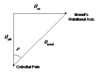
Figure 1. The Error Angle is
measured from the meridian.
Again, since we are dealing with small angular distances,
Euclidean geometry can be used and the error angle, ![]() , can be calculated as follows:
, can be calculated as follows:
![]() (7)
(7)
Why is the error angle important? The fact is that the effective polar
alignment error is dependent on where you are pointing in the sky. As an object is imaged over several minutes
or hours, the effective polar alignment error is constantly changing since the
mount is tracking in right ascension.
When you are pointing in the direction of the error angle (or 180
degrees from it), the effects of polar misalignment are minimal. Note also that pointing ![]() away from the error
angle is where you will experience the full effects of the alignment
error. We can calculate the effective
alignment error,
away from the error
angle is where you will experience the full effects of the alignment
error. We can calculate the effective
alignment error, ![]() , as:
, as:
![]() (8)
(8)
Where:
![]() is the effective
polar alignment error
is the effective
polar alignment error
![]() is the total
alignment error calculated by Equation (5)
is the total
alignment error calculated by Equation (5)
![]() is the error
angle calculated by Equation (7)
is the error
angle calculated by Equation (7)
![]() is the hour angle
where the telescope is pointing in degrees
is the hour angle
where the telescope is pointing in degrees
Notice that Equation (8) holds the key as to why the drift alignment method works. We are able to measure drift and adjust each axis independently as a consequence of this equation. When we measure azimuth error we point at the intersection of the meridian and equator. At this location the hour angle is zero. Equation (8) reduces to:
![]()
Likewise, when measuring drift in the east or west for
altitude error, the hour angle is ![]() . Equation (8) reduces
to:
. Equation (8) reduces
to:
![]()
Implications of Alignment Error Tolerance
Equation (3) carries with it some far-reaching implications that should be examined carefully. We will examine each variable in turn and look at the effect that variable has on alignment error and vice versa.
Focal Length
Focal length,![]() , is a factor in the denominator of Equation (3). Therefore, as focal length increases, the
polar alignment tolerance decreases, assuming all other factors remain
constant. This effect is predominantly
due to the image scale reduction at longer focal lengths. The star trail created by the field rotation
will occupy more pixels or film grains.
To hold
, is a factor in the denominator of Equation (3). Therefore, as focal length increases, the
polar alignment tolerance decreases, assuming all other factors remain
constant. This effect is predominantly
due to the image scale reduction at longer focal lengths. The star trail created by the field rotation
will occupy more pixels or film grains.
To hold ![]() constant, therefore,
will demand a more accurate polar alignment.
constant, therefore,
will demand a more accurate polar alignment.
We might then ask, “Given the measured alignment error, what
is the maximum focal length instrument I can use to keep field rotation within
tolerance?” To answer this, we solve
Equation (3) for ![]() :
:
![]() (9)
(9)
For example, with the parameters: alignment error = 10 arc minutes, field rotation = 9 microns, exposure time = 15 minutes, guide star angle = 3 degrees, target = 35 degrees, the calculated maximum focal length is 737 millimeters.
Guide Star Angle
Guide star angle,![]() , is a factor in the denominator of Equation (3). Therefore, as the guide star angle increases,
the polar alignment tolerance decreases, assuming all other factors remain
constant. Clearly, if you are guiding with a guide scope, try to use a guide
star as close as possible to the center of your imaging camera.
, is a factor in the denominator of Equation (3). Therefore, as the guide star angle increases,
the polar alignment tolerance decreases, assuming all other factors remain
constant. Clearly, if you are guiding with a guide scope, try to use a guide
star as close as possible to the center of your imaging camera.
Note that if you are guiding through the same optic as the
imaging device and if the guider to imaging device is rigidly fixed (as is the
case with dual sensor cameras and some off-axis guiders), the product ![]() will remain constant.
This is because in those configurations the guide star selection is
rigidly bounded and the worst case angle is inversely affected by the focal
length. For short focal lengths the
angle is larger, and inversely, the angle is smaller for larger focal lengths.
will remain constant.
This is because in those configurations the guide star selection is
rigidly bounded and the worst case angle is inversely affected by the focal
length. For short focal lengths the
angle is larger, and inversely, the angle is smaller for larger focal lengths.
To measure the guide star angle (for any configuration), try locating a star on the guider and note a star in an opposing corner of the imaging camera. If these stars can be identified in an atlas or planetarium program and their coordinates derived, the angular distance can be deduced by the following equation: [3]
![]() (10)
(10)
Where:
![]() is the angle of
separation between the two stars
is the angle of
separation between the two stars
![]() is the
declination of the first star
is the
declination of the first star
![]() is the
declination of the second star
is the
declination of the second star
![]() is the right
ascension of the first star
is the right
ascension of the first star
![]() is the right
ascension of the second star
is the right
ascension of the second star
Also remember when determining the guide star angle to take into consideration any planned cropping of the image. If the image is to be cropped (perhaps to remove some spherical aberrations) the guide star angle should be reduced accordingly, giving some relief to the polar alignment tolerance.
The relevant question here is, “Given the measured alignment
error, what is the maximum guide star angle I can use to keep field rotation
within tolerance?” To answer this, we
solve Equation (3) for ![]() :
:
![]() (11)
(11)
For example, with the parameters: alignment error = 10 arc minutes, field rotation = 9 microns, exposure time = 15 minutes, focal length = 655 mm, target = 35 degrees, the calculated maximum guide star angle is 3.38 degrees.
Exposure Time
Exposure time,![]() , is a factor in the denominator of Equation (3). Therefore, as exposure time increases, the
polar alignment tolerance decreases, assuming all other factors remain
constant. This is intuitive since the
longer we expose, the longer our star trails will become due to field rotation.
, is a factor in the denominator of Equation (3). Therefore, as exposure time increases, the
polar alignment tolerance decreases, assuming all other factors remain
constant. This is intuitive since the
longer we expose, the longer our star trails will become due to field rotation.
We might ask, “What is the longest exposure time I can make
before field rotation is noticeable?” To
answer this we solve Equation (3) for ![]() :
:
![]() (12)
(12)
For example, with the parameters: alignment error = 10 arc minutes, field rotation = 9 microns, guide star angle = 3 degrees, focal length = 655 mm, target = 35 degrees, the calculated maximum exposure time is 16.9 minutes.
Field Rotation
Field Rotation, ![]() , is a factor in the numerator of Equation (3). Therefore, as we allow for more field
rotation the polar alignment tolerance increases. Another way of looking at this is that if we
require very small star trails due to field rotation we will require a very
small polar alignment error.
, is a factor in the numerator of Equation (3). Therefore, as we allow for more field
rotation the polar alignment tolerance increases. Another way of looking at this is that if we
require very small star trails due to field rotation we will require a very
small polar alignment error.
When determining a good value to use for field rotation two rules of thumb can be applied. Some astrophotographers strive to limit the rotation to 1/3rd the minimum star size produced by their optics. So if your smallest stars are about 30 microns you might want to limit the worst case rotation to 10 microns. Another solution is to use the pixel size of your camera so that the rotation is no more than a single pixel.
Clearly, calculating the field rotation is the critical
factor of this whole exercise since it is the very variable we would like to
keep to an absolute minimum. Simply
solve Equation (3) for ![]() :
:
![]() (13)
(13)
For example, with the parameters: alignment error = 10 arc minutes, exposure time = 15 minutes, guide star angle = 3 degrees, focal length = 655 mm, target = 35 degrees, the calculated field rotation star trail is 8 microns.
Declination of the Target
Declination,![]() , is a factor in the numerator of Equation (3). Therefore, as we image closer and closer to
the celestial pole we will need a smaller and smaller alignment error. This may
not seem intuitive at first. We know
that star trails in untracked images are shorter near the pole than they are
near the equator. Why, then, do we
require more alignment accuracy near the pole?
The answer is quite simple. For
field rotation to occur there must be a correction in both declination and right ascension. The prevailing myth is that during drift
alignment there is no drift in right ascension.
This is incorrect. The drift in
right ascension when measured near the equator is very small and is usually
overwhelmed by the periodic error of the right ascension worm gear, but it does
exist in an imperfectly aligned mount and must exist for field rotation to
occur. Suppose, for a moment, that the
guiding corrections were only in the declination axis. The image would move laterally with, perhaps,
some side to side movement for periodic error, but no overall rotation would
occur. However, this is simply not the
case in an imperfectly polar aligned mount.
Over time a small drift in right ascension will cause field rotation.
, is a factor in the numerator of Equation (3). Therefore, as we image closer and closer to
the celestial pole we will need a smaller and smaller alignment error. This may
not seem intuitive at first. We know
that star trails in untracked images are shorter near the pole than they are
near the equator. Why, then, do we
require more alignment accuracy near the pole?
The answer is quite simple. For
field rotation to occur there must be a correction in both declination and right ascension. The prevailing myth is that during drift
alignment there is no drift in right ascension.
This is incorrect. The drift in
right ascension when measured near the equator is very small and is usually
overwhelmed by the periodic error of the right ascension worm gear, but it does
exist in an imperfectly aligned mount and must exist for field rotation to
occur. Suppose, for a moment, that the
guiding corrections were only in the declination axis. The image would move laterally with, perhaps,
some side to side movement for periodic error, but no overall rotation would
occur. However, this is simply not the
case in an imperfectly polar aligned mount.
Over time a small drift in right ascension will cause field rotation.
The situation is unique near the pole. Near the pole the correction required for right ascension is more significant than is needed at the equator given the same polar alignment error and will result in more field rotation when guiding. Why? At the equator the movement due to correction is predominately linear. The declination error is greater than the right ascension error. Near the pole the movement is more circular and the correction in right ascension is more significant. It is this increase in right ascension correction that causes the rotation to be more severe at the polar regions. The illustration in Figure 2 may make this clearer. Here position A represents the star’s starting position, B is where the misaligned mount would point after some period, and C is where the mount should be pointing if it were perfectly aligned. Note also that for illustration purposes the alignment error near the equator is exaggerated; still you can see that the correction in right ascension is relatively small. This correction amount will decrease significantly as the error angle is decreased.
The implication here is clear; if we are going to image at
declinations near the celestial poles we will require very tight alignment
tolerances. The other alternative is to
attempt to image unguided since star trailing near the pole should not be too
offensive and may fall below our tolerance, ![]() .
.
So how do we calculate the maximum declination given our
measured alignment error? The answer
requires us to solve Equation (3) for ![]() :
:
![]() (14)
(14)
For example, with the parameters: alignment error = 10 arc minutes, exposure time = 15 minutes, guide star angle = 3 degrees, focal length = 655 mm, field rotation = 9 microns, the calculated maximum declination is 64.1 degrees.
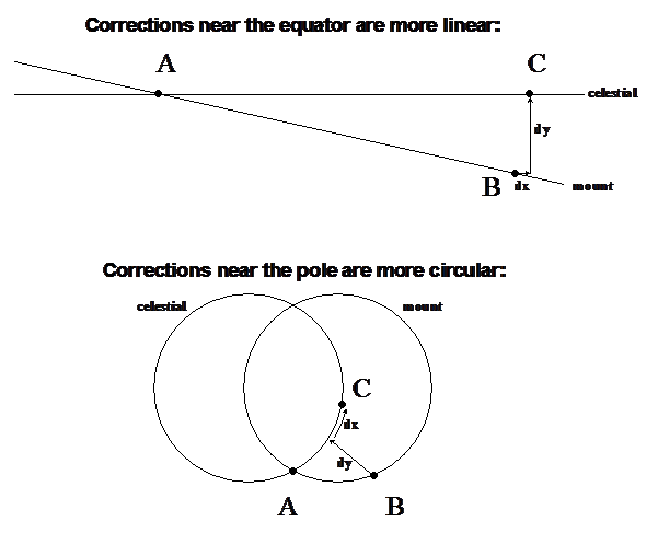
Figure 2. Field rotation is more
severe near the poles due to more significant corrections in R.A.
Conclusions
With the mathematical model disclosed here, we have at our disposal the means to determine the polar alignment error of our equatorially mounted instruments. Armed with this information, we can also determine if the alignment error is within acceptable tolerances for the imaging session.
It is hoped that this narrative will take some of the mystery out of the polar alignment procedure. The information presented here can be used as an important aid to the normal drift alignment procedure. Having the ability to quantify the polar alignment error may reduce the time for accurate alignment by making the axes adjustments in a more deterministic, data-driven fashion.
The implications of the various factors affecting alignment error tolerance provide the astrophotographer with intelligent alternatives. If the measured alignment error is insufficient given the calculated tolerance for error the choice can be made to:
· Reduce the exposure time
· Find an image target at a lower declination
· Choose a guide star closer to the target
· Allow for more field rotation
· Image with a shorter focal length
· Adjust the mount to improve the polar alignment.
References
[1] MacRobert, A., Accurate Polar Alignment, (2006)
http://www.skyandtelescope.com/astronomy-resources/accurate-polar-alignment/
[2] Hook, R.N., Polar axis alignment requirements of astronomical photography,
Journal of the British Astronomical Association, vol. 99, no. 1, p. 19-22 (Feb. 1989)
[3] Meeus, J., Astronomical Algorithms, 2nd Edition, (1998)
Chapter 17, “Angular Separation”
[4] Barrett, F.A., Measuring Polar Axis Alignment Error,
(2016)
http://celestialwonders.com/articles/polaralignment/MeasuringAlignmentError.html